

This post originally appeared on the In The Loupe blog.
Tolerance stacking, also known as tolerance stack-up, refers to the combination of various part dimension tolerances. After a tolerance is identified on the dimension of a part, it is important to test whether that tolerance would work with the tool’s tolerances: either the upper end or lower end. A part or assembly can be subject to inaccuracies when its tolerances are stacked up incorrectly.
The Importance of Tolerances
Tolerances directly influence the cost and performance of a product. Tighter tolerances make a machined part more difficult to manufacture and therefore often more expensive. With this in mind, it is important to find a balance between manufacturability of the part, its functionality, and its cost.
Tips for Successful Tolerance Stacking
Avoid Using Tolerances that are Unnecessarily Small
As stated above, tighter tolerances lead to a higher manufacturing cost as the part is more difficult to make. This higher cost is often due to the increased amount of scrapped parts that can occur when dimensions are found to be out of tolerance. The cost of high quality tool holders and tooling with tighter tolerances can also be an added expense.
Additionally, unnecessarily small tolerances will lead to longer manufacturing times, as more work goes in to ensure that the part meets strict criteria during machining, and after machining in the inspection process.
Be Careful Not to Over Dimension a Part
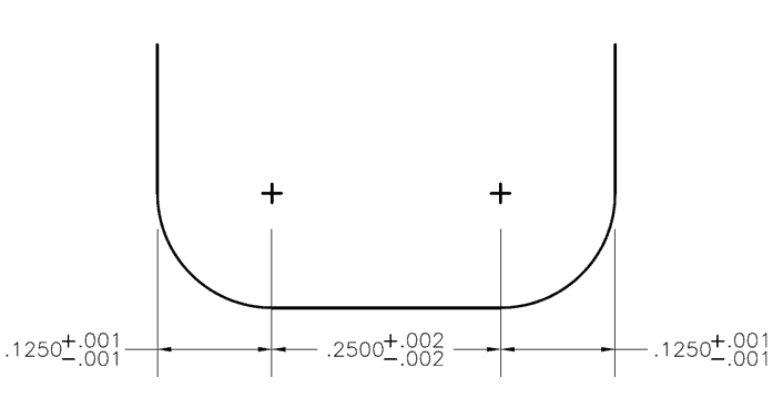
When an upper and lower tolerance is labeled on every feature of a part, over-dimensioning can become a problem. For example, a corner radius end mill with a right and left corner radii might have a tolerance of +/- .001”, and the flat between them has a .002” tolerance. In this case, the tolerance window for the cutter diameter would be +/- .004”, but is oftentimes miscalculated during part dimensioning. Further, placing a tolerance on this callout would cause it to be over dimensioned, and thus the reference dimension “REF” must be left to take the tolerance’s place.
Image Caption: Figure 1: Shape of slot created by a corner radius end mill
Utilize Statistical Tolerance Analysis:
Statistical analysis looks at the likelihood that all three tolerances would be below or above the dimensioned slot width, based on a standard deviation. This probability is represented by a normal probability density function, which can be seen in figure 2 below. By combining all the probabilities of the different parts and dimensions in a design, we can determine the probability that a part will have a problem, or fail altogether, based on the dimensions and tolerance of the parts. Generally this method of analysis is only used for assemblies with four or more tolerances.
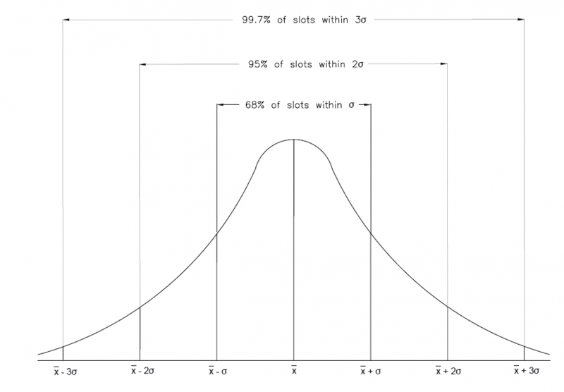
Image caption: Figure 2: Tolerance Stacking: Normal distribution
Before starting a statistical tolerance analysis, you must calculate or choose a tolerance distribution factor. The standard distribution is 3. This means that most of the data (or in this case tolerances) will be within 3 standard deviations of the mean. The standard deviations of all the tolerances must be divided by this tolerance distribution factor to normalize them from a distribution of 3 to a distribution of 1. Once this has been done, the root sum squared can be taken to find the standard deviation of the assembly.
Think of it like a cup of coffee being made with 3 different sized beans. In order to make a delicious cup of joe, you must first grind down all of the beans to the same size so they can be added to the coffee filter. In this case, the beans are the standard deviations, the grinder is the tolerance distribution factor, and the coffee filter is the root sum squared equation. This is necessary because some tolerances may have different distribution factors based on the tightness of the tolerance range.
The statistical analysis method is used if there is a requirement that the slot must be .500” wide with a +/- .003” tolerance, but there is no need for the radii (.125”) and the flat (.250”) to be exact as long as they fit within the slot. In this example, we have 3 bilateral tolerances with their standard deviations already available. Since they are bilateral, the standard deviation from the mean would simply be whatever the + or – tolerance value is. For the outside radii, this would be .001” and for the middle flat region this would be .002”.
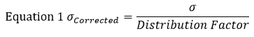
For this example, let’s find the standard deviation (σ) of each section using equation 1. In this equation represents the standard deviation.
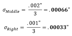
The standard assumption is that a part tolerance represents a +/- 3 normal distribution. Therefore, the distribution factor will be 3. Using equation 1 on the left section of figure 1, we find that its corrected standard deviation equates to:
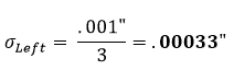
This is then repeated for the middle and right sections:
After arriving at these standard deviations, we input the results into equation 2 to find the standard deviation of the tolerance zone. Equation 2 is known as the root sum squared equation.
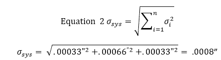
At this point, it means that 68% of the slots will be within a +/- .00122” tolerance. Multiplying this tolerance by 2 will result in a 95% confidence window, where multiplying it by 3 will result in a 99% confidence window.
68% of the slots will be within +/- .0008”
95% of the slots will be within +/- .0016”
99% of the slots will be within +/- .0024”
These confidence windows are standard for a normal distributed set of data points. A standard normal distribution can be seen in Figure 2 above.
Statistical tolerance analysis should only be used for assemblies with greater than 4 toleranced parts. A lot of factors were unaccounted for in this simple analysis. This example was for 3 bilateral dimensions whose tolerances were representative of their standard deviations from their means. In standard statistical tolerance analysis, other variables come into play such as angles, runout, and parallelism, which require correction factors.
Use Worst Case Analysis:
Worst case analysis is the practice of adding up all the tolerances of a part to find the total part tolerance. When performing this type of analysis, each tolerance is set to its largest or smallest limit in its respective range. This total tolerance can then be compared to the performance limits of the part to make sure the assembly is designed properly. This is typically used for only 1 dimension (Only 1 plane, therefore no angles involved) and for assemblies with a small number of parts.
Worst case analysis can also be used when choosing the appropriate cutting tool for your job, as the tool’s tolerance can be added to the parts tolerance for a worst case scenario. Once this scenario is identified, the machinist or engineer can make the appropriate adjustments to keep the part within the dimensions specified on the print. It should be noted that the worst case scenario rarely ever occurs in actual production. While these analyses can be expensive for manufacturing, it provides peace of mind to machinists by guaranteeing that all assemblies will function properly. Often this method requires tight tolerances because the total stack up at maximum conditions is the primary feature used in design. Tighter tolerances intensify manufacturing costs due to the increased amount of scraping, production time for inspection, and cost of tooling used on these parts.
Example of worst case scenario in context to Figure 1:
Find the lower specification limit.
For the left corner radius
.125” - .001” = .124”
For the flat section
.250” - .002” = .248”
For the right corner radius
.125” - .001” = .124”
Add all of these together to the lower specification limit:
.124” + .248” + .124” = .496”
Find the upper specification limit:
For the left corner radius
.125” + .001” = .126”
For the flat section
.250” + .002” = .252”
For the right corner radius
.125” + .001” = .126”
Add all of these together to the lower specification limit:
.126” + .252” + .126” = .504”
Subtract the two and divide this answer by two to get the worst case tolerance:
(Upper Limit – Lower Limit)/2 = .004”
Therefore the worst case scenario of this slot is .500” +/- .004”.